Making documents with makefiles

I learned to use the command line utility make in the context of building C programs. The program make reads an input file to tell it how to make things. To make a C program, you compile the source files into object files, then link the object files together.

You can tell make what depends on what, so it will not do any unnecessary work. If you tell it that a file foo.o depends on a file foo.c, then it will rebuild foo.o if that file is older than the file foo.c that it depends on. Looking at file timestamps allows make to save time by not doing unnecessary work. It also makes it easier to dictate what order things need to be done in.

There is nothing about make that is limited to compiling programs. It simply orchestrates commands in a declarative way. Because you state what the dependencies are, but let it figure if and when each needs to be run, a makefile is more like a Prolog program than a Python script.

I have a client that needs a dozen customized reports, each of which requires a few steps to create, and the order of the steps is important. I created the reports by hand. Then, of course, something changed and all the reports needed to be remade. So then I wrote a Python script to manage the next build. (And the next, and the next, …). But I should have written a makefile. I’m about to have to revise the reports, and this time I’ll probably use a makefile.

Here’s a very simple example of using a makefile to create documents. For more extensive examples of how to use makefiles for a variety of tasks, see How I stopped worrying and loved Makefiles. [1]

Suppose you need to create a PDF and a Microsoft Word version of a report from a LaTeX file [2].

all: foo.pdf foo.docx

foo.pdf: foo.tex
	pdflatex foo.tex

foo.docx: foo.tex
	pandoc foo.tex --from latex --to docx > foo.docx

clean:
	rm foo.aux foo.log

If the file foo.pdf does not exist, or exists but it older than foo.tex, the command make foo.pdf will create the PDF file by running pdflatex. If foo.pdf is newer than foo.tex then running make foo.pdf will return a message

make: 'foo.pdf' is up to date.

If you run make with no argument, it will build both foo.pdf and foo.docx as needed.

The command make clean deletes auxiliary files created by pdflatex. This shows that a make action does have to “make” anything; it simply runs a command.


[1] The blog post title is an allusion to the 1964 movie Dr. Strangelove or: How I Learned to Stop Worrying and Love the Bomb.

[2] I use LaTeX for everything I can. This saves time in the long run, if not in the moment, because of consistency. I used to use Word for proposals and such, and LaTeX for documents requiring equations. My workflow became more efficient when I switched to using LaTeX for everything.

Applied abstraction

“Good general theory does not search for the maximum generality, but for the right generality.” — Saunders Mac Lane


One of the benefits of a scripting language like Python is that it gives you generalizations for free. For example, take the function sorted. If you give it a list of integers, it will return a list of numerically sorted integers. But you could also give it a list of strings, and it will return a list of alphabetically sorted strings. In fact, you can give it more general collections of more general things. The user gets generality for free: more functionality without complicating the syntax for the most concrete use case.

Here’s a similar example in math. Suppose you prove that for invertible matrices A and B of the same size

(AB)−1 = B−1 A−1.

You can prove just as easily that the same is true for any elements A and B in a group. In fact, the proof may be simpler. Because you have less to work with in a group, you’re lead by the nose to a simple proof.

But not all generalizations are free. In the sorting example, suppose you want your code to do more than sort lists, but instead perform any operation on lists that satisfies some properties that sorting has. This is the kind of thing some Haskell programmers love to do. The result is a kind of impenetrable code that takes talent to write.

Mathematical theorems are usually discovered in some concrete setting, then codified in a more general setting. There is some optimal level of generality that clarifies the original discovery without introducing more difficulty. But it is possible to push past this degree of generality at the cost of less intuitive hypotheses and more complicated proofs. The generalization comes at a cost. The cost may be worthwhile or not, depending on one’s motivations.

A gratuitous abstraction is one that has no apparent benefit and comes at some cost. A gratuitous abstraction may turn out to be useful in the future, but this rarely happens. And if it does happen, it will likely be because someone was lead to re-discover the abstract result while pursuing a particular problem, not because they read the abstract result and thought of an application.

This post was motivated by looking at generalizations of the Möbius inversion formula. Mr. Möbius introduced his formula nearly two centuries ago in the context of a concrete problem in number theory. The formula has been greatly generalized since then in ways that would appear to be gratuitous, introducing incidence algebras and so forth. But these generalizations have made the formula more widely applicable, particularly to problems in combinatorics.

I won’t get into Möbius inversion now, but I may in the future. Here is a post I wrote a couple years ago that touches on Möbius inversion.

I was uncritical of generalization as an undergrad. Striving for maximum generality was fine with me. Then I hit my abstraction tolerance in grad school, and became leery of gratuitous abstraction. I’ve been disappointed by going down highly abstract rabbit holes that never paid off. But Möbius inversion reminds me that levels of abstraction that seem gratuitous may be practical after all.

Posts on abstraction tolerance

A deck of cards

One time when I was in grad school, I was a teaching assistant for a business math class that included calculus and a smattering of other topics, including a little bit of probability. I made up examples involving a deck of cards, but then learned to my surprise that not everyone was familiar with playing cards. I was young and had a lot to learn about seeing things through the eyes of other people.

Later I learned that a “standard” deck of cards is not quite as standard as I thought. The “standard 52-card deck” is indeed standard in the English-speaking world, but there are variations used in other countries.

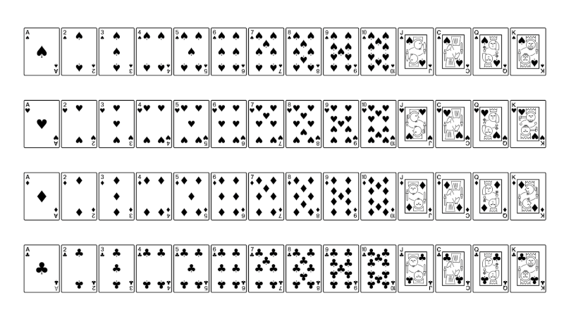
The Unicode values for the characters representing playing cards are laid out in a nice pattern. The last digit of the Unicode value corresponds to the point value of the card (aces low), and the second-to-last digit corresponds to the suite.

The ace of spades has code point U+1F0A1, and the aces of hearts, diamonds, and clubs have values  U+1F0B1, U+1F0C1, and U+1F0D1 respectively. The three of spades is U+1F0A3 and the seven of hearts is U+1F0B7.

But there’s a surprise if you’re only away of the standard 52-card deck: there’s a knight between the jack and the queen. The Unicode values for jacks end in B (Bhex = 11ten) as you’d expect, but queens end in D and kings end in E. The cards ending in C are knights, cards that don’t exist in the standard 52-card deck.

Here’s a little Python code that illustrates the Unicode layout.

for i in range(4):
   for j in range(14):
     print(chr(0x1f0a1+j+16*i), end='')
   print()

The output is too small to read as plain text, but here’s a screen shot from running the code above in a terminal with a huge font.

Unicode cards

Playing cards have their origin in tarot cards, which are commonly associated with the occult. But John C. Wright argues that tarot cards were based on Christian iconography before they became associated with the occult.

What can JWST see?

The other day I ran across this photo of Saturn’s moon Titan taken by the James Webb Space Telescope (JWST).

If JWST can see Titan with this kind of resolution, how well could it see Pluto or other planets? In this post I’ll do some back-of-the-envelope calculations, only considering the apparent size of objects, ignoring other factors such as how bright an object is.

The apparent size of an object of radius r at a distance d is proportional to (r/d)². [1]

Of course the JWST isn’t located on Earth, but JWST is close to Earth relative to the distance to Titan.

Titan is about 1.4 × 10¹² meters from here, and has a radius of about 2.6 × 10⁶ m. Pluto is about 6 × 10¹² m away, and has a radius of 1.2 × 10⁶ m. So the apparent size of Pluto would be around 90 times smaller than the apparent size of Titan. Based on only the factors considered here, JWST could take a decent photo of Pluto, but it would be lower resolution than the photo of Titan above, and far lower resolution than the photos taken by New Horizons.

Could JWST photograph an exoplanet? There are two confirmed exoplanets are orbiting Proxima Centauri 4 × 10¹⁶ m away. The larger of these has a mass slightly larger than Earth, and presumably has a radius about equal to that of Earth, 6 × 10⁶ m. Its apparent size would be 150 million times smaller than Titan.

So no, it would not be possible for JWST to photograph an expolanet.


[1] In case the apparent size calculation feels like a rabbit out of a hat, here’s a quick derivation. Imagine looking out on sphere of radius d. This sphere has area 4πd². A distant planet takes up πr² area on this sphere, 0.25(r/d)² of your total field of vision.

Fizz buzz walk

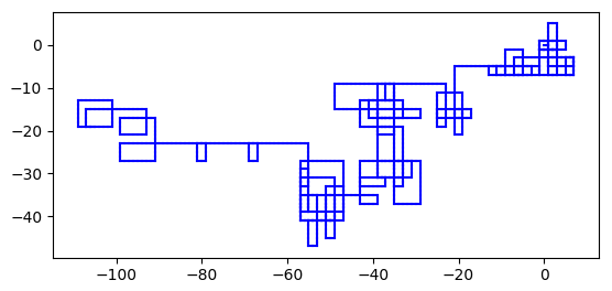
I ran across a graphic yesterday made by taking a sequence of steps of the same length, turning left on the nth step if n is prime, and otherwise continuing in the same direction.

Here’s my recreation of the first 1000 steps:

You can see that in general it makes a lot of turns at first and then turns less often as the density of primes thins out.

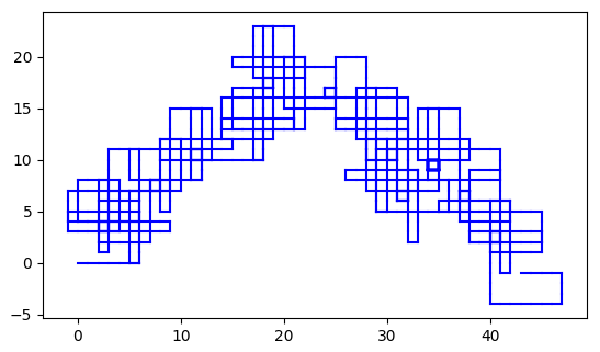
I wondered what the analogous walk would look like for Fizz Buzz. There are several variations on Fizz Buzz, and the one that produced the most interesting visualization was to turn left when a number either is divisible by 7 or contains the digit 7.

Here’s what that looks like:

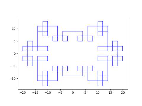
I wrote about something similar four years ago using a different rule for turning. That post looks at a walk on the complex numbers, turning left when you land on a Gaussian prime, a generalization of primes for complex numbers. These images have more symmetry and form closed loops. For example, here’s the walk you get starting at 3 + 5i.

starting at 3 + 5i

The starting point matters. See the earlier post for more examples with different starting points.

Related posts

Closed-form solutions to nonlinear PDEs

The traditional approach to teaching differential equations is to present a collection of techniques for finding closed-form solutions to ordinary differential equations (ODEs). These techniques seem completely unrelated [1] and have arcane names such as integrating factors, exact equations, variation of parameters, etc.

Students may reasonably come away from an introductory course with the false impression that it is common for ODEs to have closed-form solutions because it is common in the class.

My education reacted against this. We were told from the beginning that differential equations rarely have closed-form solutions and that therefore we wouldn’t waste time learning how to find such solutions. I didn’t learn the classical solution techniques until years later when I taught an ODE class as a postdoc.

I also came away with a false impression, the idea that differential equations almost never have closed-form solutions in practice, especially nonlinear equations, and above all partial differential equations (PDEs). This isn’t far from the truth, but it is an exaggeration.

I specialized in nonlinear PDEs in grad school, and I don’t recall ever seeing a closed-form solution. I heard rumors of a nonlinear PDE with a closed form solution, the KdV equation, but I saw this as the exception that proves the rule. It was the only nonlinear PDE of practical importance with a closed-form solution, or so I thought.

It is unusual for a nonlinear PDE to have a closed-form solution, but it is not unheard of. There are numerous examples of nonlinear PDEs, equations with important physical applications, that have closed-form solutions.

Yesterday I received a review copy of Analytical Methods for Solving Nonlinear Partial Differential Equations by Daniel Arrigo. If I had run across with a book by that title as a grad student, it would have sounded as eldritch as a book on the biology of Bigfoot or the geography of Atlantis.

A few pages into the book there are nine exercises asking the reader to verify closed-form solutions to nonlinear PDEs:

  1. a nonlinear diffusion equation
  2. Fisher’s equation
  3. Fitzhugh-Nagumo equation
  4. Berger’s equation
  5. Liouville’s equation
  6. Sine-Gordon equation
  7. Korteweg–De Vries (KdV) equation
  8. modified Korteweg–De Vries (mKdV) equation
  9. Boussinesq’s equation

These are not artificial examples crafted to have closed-form solutions. These are differential equations that were formulated to model physical phenomena such as groundwater flow, nerve impulse transmission, and acoustics.

It remains true that differential equations, and especially nonlinear PDEs, typically must be solved numerically in applications. But the number of nonlinear PDEs with closed-form solutions is not insignificant.

Related posts

[1] These techniques are not as haphazard as they seem. At a deeper level, they’re all about exploiting various forms of symmetry.


Choosing a Computer Language for a Project

Julia. Scala. Lua. TypeScript. Haskell. Go. Dart. Various computer languages new and old are sometimes proposed as better alternatives to mainstream languages. But compared to mainstream choices like Python, C, C++ and Java (cf. Tiobe Index)—are they worth using?

Certainly it depends a lot on the planned use: is it a one-off small project, or a large industrial-scale software application?

Yet even a one-off project can quickly grow to production-scale, with accompanying growing pains. Startups sometimes face a growth crisis when the nascent code base becomes unwieldy and must be refactored or fully rewritten (or you could do what Facebook/Meta did and just write a new compiler to make your existing code base run better).

The scope of different types of software projects and their requirements is so incredibly diverse that any single viewpoint from experience runs a risk of being myopic and thus inaccurate for other kinds of projects. With this caveat, I’ll share some of my own experience from observing projects for many dozens of production-scale software applications written for leadership-scale high performance computing systems. These are generally on a scale of 20,000 to 500,000 lines of code and often require support of mathematical and scientific libraries and middleware for build support, parallelism, visualization, I/O, data management and machine learning.

Here are some of the main issues regarding choice of programming languages and compilers for these codes:

1. Language and compiler sustainability. While the lifetime of computing systems is measured in years, the lifetime of an application code base can sometimes be measured in decades. Is the language it is written in likely to survive and be well-supported long into the future? For example, Fortran, though still used and frequently supported, is is a less common language thus requiring special effort from vendors, with fewer developer resources than more popular languages. Is there a diversity of multiple compilers from different providers to mitigate risk? A single provider means a single point of failure, a high risk; what happens if the supplier loses funding? Are the language and compilers likely to be adaptable for future computer hardware trends (though sometimes this is hard to predict)? Is there a large customer base to help ensure future support? Similarly, is there an adequate pool of available programmers deeply skilled in the language? Does the language have a well-featured standard library ecosystem and good support for third-party libraries and frameworks? Is there good tool support (debuggers, profilers, build tools)?

2. Related to this is the question of language governance. How are decisions about future updates to the language made? Is there broad participation from the user community and responsiveness to their needs? I’ve known members of the C++ language committee; from my limited experience they seem very reasonable and thoughtful about future directions of the language. On the other hand, some standards have introduced features that scarcely anyone ever uses—a waste of time and more clutter for the standard.

3. Productivity. It is said that programmer productivity is limited by the ability of a few lines of code to express high level abstractions that can do a lot with minimal syntax. Does the language permit this? Does the language standard make sense (coherent, cohesive) and follow the principle of least surprise? At the same time, the language should not engulf what might better be handled modularly by a library. For example, a matrix-matrix product that is bound up with the language might be highly productive for simple cases but have difficulty supporting the many variants of matrix-matrix product provided for example by the NVIDIA CUTLASS library. Also, in-language support for CUDA GPU operations, for example, would make it hard for the language not to lag behind in support of the frequent new releases of CUDA.

4. Strategic advantage. The 10X improvement rule states that an innovation is only worth adopting if it offers 10X improvement compared to existing practice according to some metric . If switching to a given new language doesn’t bring significant improvement, it may not be worth doing. This is particularly true if there is an existing code base of some size. A related question is whether the new language offers an incremental transition path for an existing code to the new language (in many cases this is difficult or impossible).

5. Performance (execution speed). Does the language allow one to get down to bare-metal performance rather than going through costly abstractions or an interpreter layer? Are the features of the underlying hardware exposed for the user to access? Is performance predictable? Can one get a sense of the performance of each line of code just by inspection, or is this occluded by abstractions or a complex compilation process? Is the use of just-in-time compilation or garbage collection unpredictable, which could be a problem for parallel computing wherein unexpected “hangs” can be caused by one process unexpectedly performing one of these operations? Do the compiler developers provide good support for effective and accurate code optimization options? Have results from standardized non-cherry-picked benchmarks been published (kernel benchmarks, proxy apps, full applications)?

Early adopters provide a vibrant “early alert” system for new language and tool developments that are useful for small projects and may be broadly impactful. Python was recognized early in the scientific computing community for its potential complementary use with standard languages for large scientific computations. When it comes to planning large-scale software projects, however, a range of factors based on project requirements must be considered to ensure highest likelihood of success.


On greedy algorithms and rodeo clowns

Rodeo clown

This weekend I ran across a blog post The Rodeo Clown Theory of Personal Development. The title comes from a hypothetical example of a goal you don’t know how to achieve: becoming a rodeo clown.

Let’s say you decide you want to be a rodeo clown. And let’s say you’re me and you have no idea how to be a rodeo clown. … Can you look at the possibilities currently available to you and imagine which of them might lead to an overall increase of rodeo clowndom in your life, even infinitesimally?

Each day you ask yourself what you can do that might lead you closer to your goal. This is a greedy algorithm: at each step you make as much progress toward your goal as you can. Greedy algorithms are not always optimal, but the premise above is that you have no idea what to do. In that case, doing whatever you can imagine that might bring you a little closer to your goal is a smart thing to do.

Crossing the continent

If you’re in Los Angeles and your goal is to get to New York, you could start by walking east. You might run into a brick wall and decide that you should not take your approach too literally. Maybe you decide to buy a ticket for a bus that’s traveling east, even if you have to walk west to the bus station. Maybe the bus takes you to Houston. This isn’t the most direct route, but it’s progress.

When you don’t know what else to do, a greedy approach, especially one tempered with common sense, could be a very sensible way to start. Maybe it’ll put you in a position to learn of a more efficient approach. In the scenario above, maybe some stranger sees you walk into a wall, asks you what you’re trying to do, and tells you where the bus station is.

Sorting algorithms

The way most people sort a hand of playing cards is a sort of greedy algorithm. They scan for the highest card and put it first. Then they scan the remainder of the hand for the next highest card and so on. This algorithm is known as insertion sort. It’s not the most efficient algorithm, but it may be the most natural, and it works. And for a hand of five cards it’s about as good as any.

Anyone who has taken an algorithms class will know you can beat insertion sort with a more sophisticated algorithm such as heap sort. But sorting is a well-understood, one-dimensional problem. That’s why people long ago came up with solutions that are better than a greedy approach. But when a problem is not well understood and is high-dimensional, greedy algorithms are more likely to succeed, even if they’re not optimal.

Training neural nets

Training a neural network is a very high dimensional optimization problem, maybe on the order of a billion dimensions. And yet it is solved using stochastic gradient descent, which is essentially a greedy algorithm. At each iteration, you move in the direction that gives you the most improvement toward your goal. There’s a little more nuance to it than that, but that’s the basic idea.

How can gradient descent work so well in practice when in theory it could get stuck in a local minimum or a saddle point? John Carmack posted a heuristic explanation on Twitter a few weeks ago. A local critical point requires the “cooperation” of every variable in the function you’re optimizing. The more variables, the less likely this is to happen.

Carmack didn’t give a full explanation—he posted a tweet, not a journal article—but he does give an intuitive idea of what’s going on. At the global minimum, the variables cooperate for a good reason. He assumes the variables are unlikely to cooperate anywhere else, which is apparently often true when training neural nets.

Usually things get harder in higher dimensions, hence the “curse of dimensionality.” But there’s a sort of blessing of dimensionality here: you’re less likely to get stuck in a local minimum in higher dimensions.

Back to the rodeo

Training a neural network can be a huge undertaking, using millions of dollars worth of electricity, but it’s a mathematically defined problem. Life goals such as becoming a rodeo clown are not cleanly quantified problems. They are very high dimensional in the sense that there are a vast number of things you could do at any given time. You might argue by analogy with neural nets that the fact that there are so many dimensions means that you’re unlikely to get stuck in a local minimum. This is a loose analogy, one that easily breaks down, but still one worth thinking about.

Seth Godin once said “Remarkable work often comes from making choices when everyone else feels as though there is no choice.” What looks like a local minimum may be revealed to not be once you consider more options.


Image by Clarence Alford from Pixabay

Finding strings in binary files

There’s a little program called strings that searches for what appear to be strings inside binary file. I’ll refer to it as strings(1) to distinguish the program name from the common English word strings. [1]

What does strings(1) consider to be a string? By default it is a sequence of four or more bytes that correspond to printable ASCII strings. There are command options to change the sequence length and the character encoding.

There are 98 printable ASCII characters [2] and 256 possible values for an 8-bit byte, so the probability of a byte being a printable character is

p = 98/256 = 0.3828125.

This implies that the probability of strings(1) flagging a sequence of four random bytes as a string is p4 or about 2%.

How long a string might you find inside a binary file?

I ran strings(1) on a photograph and found a 46-character string:

   .IEC 61966-2.1 Default RGB colour space - sRGB

Of course this isn’t random. This string is part of the metadata stored inside JPEG images.

Next I encrypted the file so that no strings would be metadata and all strings would be false positives. The longest line was 12 characters:

    Z<Bq{7fH}~G9

How does this compare to what we might expect from a random file? I wrote about the probability of long runs a dozen years ago. In a file of n bytes, the expected length of the longest run of printable characters is approximately

-frac{log n(1-p)}{log p}

In my case, the file had n = 203,308 bytes. The expected length of the longest run of printable characters would then be 12.2 characters, and so the actual length of the longest run is in line with what theory would have predicted.


[1] Unix documentation is separated into sections, and parentheses after a name specify the documentation section. Section 1 is for programs, Section 2 is for system calls, etc. So, for example, chmod(1) is the command line utility named chmod, and chmod(2) is the system call by the same name. Since command line utilities often have names that are common words, tacking (1) on the end helps distinguish program names from English words.

[2] p could be a little larger if you consider some of the control characters to be printable.

Extract text from a PDF

Arshad Khan left a comment on my post on the less and more utilities saying “on ubuntu if I do less on a pdf file, it shows me the text contents of the pdf.”

Apparently this is an undocumented feature of GNU less. It works, but I don’t see anything about it in the man page documentation [1].

Not all versions of less do this. On my Mac, less applied to a PDF gives a warning saying “… may be a binary file. See it anyway?” If you insist, it will dump gibberish to the command line.

A more portable way to extract text from a PDF would be to use something like the pypdf Python module:

    from pypdf import PdfReader

    reader = PdfReader("myfile.pdf")
    for page in reader.pages:
        print(page.extract_text()) 

The pypdf documentation gives several options for how to extract text. The documentation also gives a helpful discussion of why it’s not always clear what extracting text from a PDF should mean. Should captions and page numbers be extracted? What about tables? In what order should text elements be extracted?

PDF files are notoriously bad as a data exchange format. When you extract text from a PDF, you’re likely not using the file in a way its author intended, maybe even in a way the author tried to discourage.

Related post: Your PDF may reveal more than you intend

[1] Update: Several people have responded saying that that less isn’t extracting the text from a PDF, but lesspipe is. That would explain why it’s not a documented feature of less. But it’s not clear how lesspipe is implicitly inserting itself.

Further update: Thanks to Konrad Hinsen for pointing me to this explanation. less reads an environment variable LESSOPEN for a preprocessor to run on its arguments, and that variable is, on some systems, set to lesspipe.