3d Glitching Notes – Part 4 – Texture Map Glitching…

As with the earlier notes, this will make more sense if you have some prior knowledge of 3d modeling and rendering (and, in this case, texture mapping). A knowledge of Blender will be especially useful. Hopefully you can make the necessary adjustments if you use a different 3d modeling and rendering application. It’s assumed that  you’ve gone through the previous  notes in this series, starting here .

So far I’ve discussed glitching the 3d vertices of a model described in an .obj file. These vertices define the object’s surface in 3d space. However, the file can also contain a list of texture vertices, sometimes referred to as UV vertices. These allow a 2d image to be mapped to a 3d surface in the same way that a Mercator projection map corresponds to a globe, or the way the flattened, peeled skin of an orange can be fitted back onto the orange.

In this note I’ll discuss the first of several approaches to “glitching” the way a texture is mapped to a 3d object. This first method hews more closely to the original glitch esthetic in that the results are mostly a matter of chance. We’ll open an .obj file, cut and paste, find and replace, and discover afterwards what the effects are.

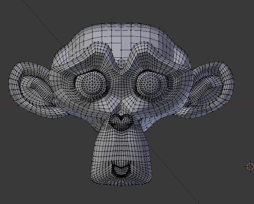
Something else that will be different about this set of notes: Instead of working with a mesh that is fully rounded – a model of a head, for example – I’ll use a flat mesh and show how the final product of this method of glitching can be another 2d image. However, everything I explain here applies equally to the texturing of 3d models of the more usual, fully rounded type.

I won’t go into the technical details of the structure of an .obj file or  how the texture mapping takes place.. all that is available on the web and has been discussed to some degree in the previous notes. For now, just know that the texture vertices in an object file are on the lines that begin with the characters “vt”.

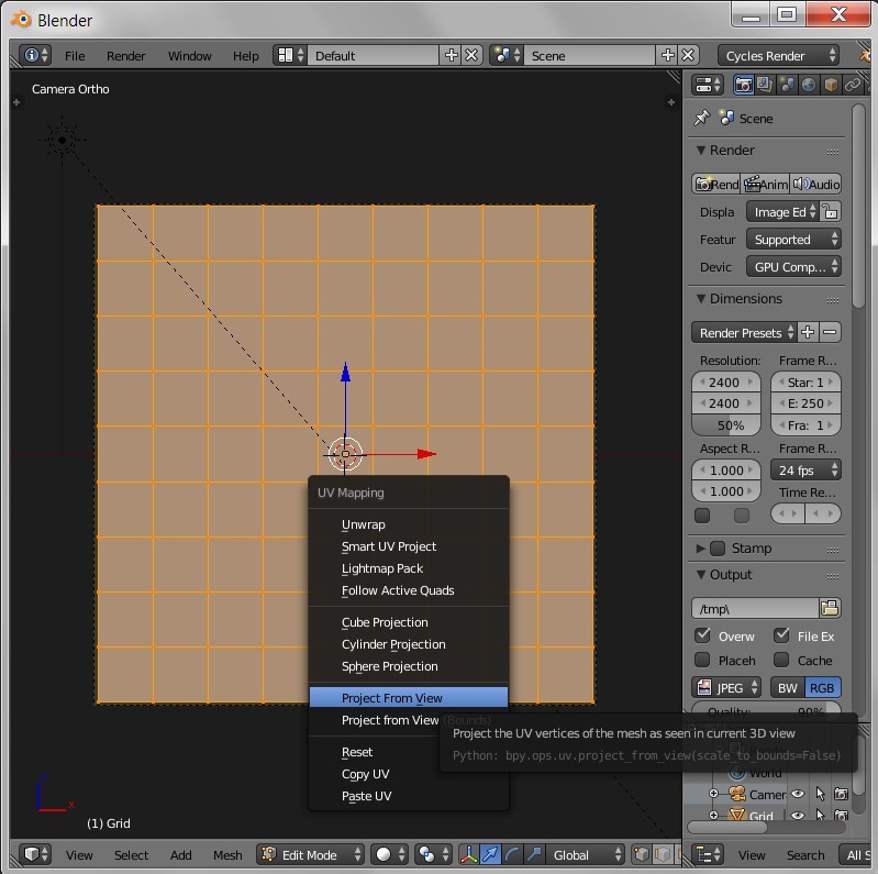
Our first job is to obtain an .obj file with texture vertices. In Blender, we create a 2d grid, set up an orthographic camera, and align it so the camera view is perpendicular to and facing the grid. We then go into “Edit” mode, select all the vertices of the grid, and hit the “u” key on the keyboard (stands for “unwrap”). From the available choices, pick “Project from View”. That’s it.


01uvUnwrap


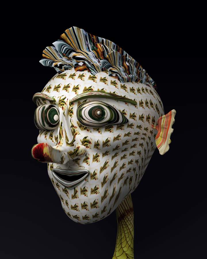
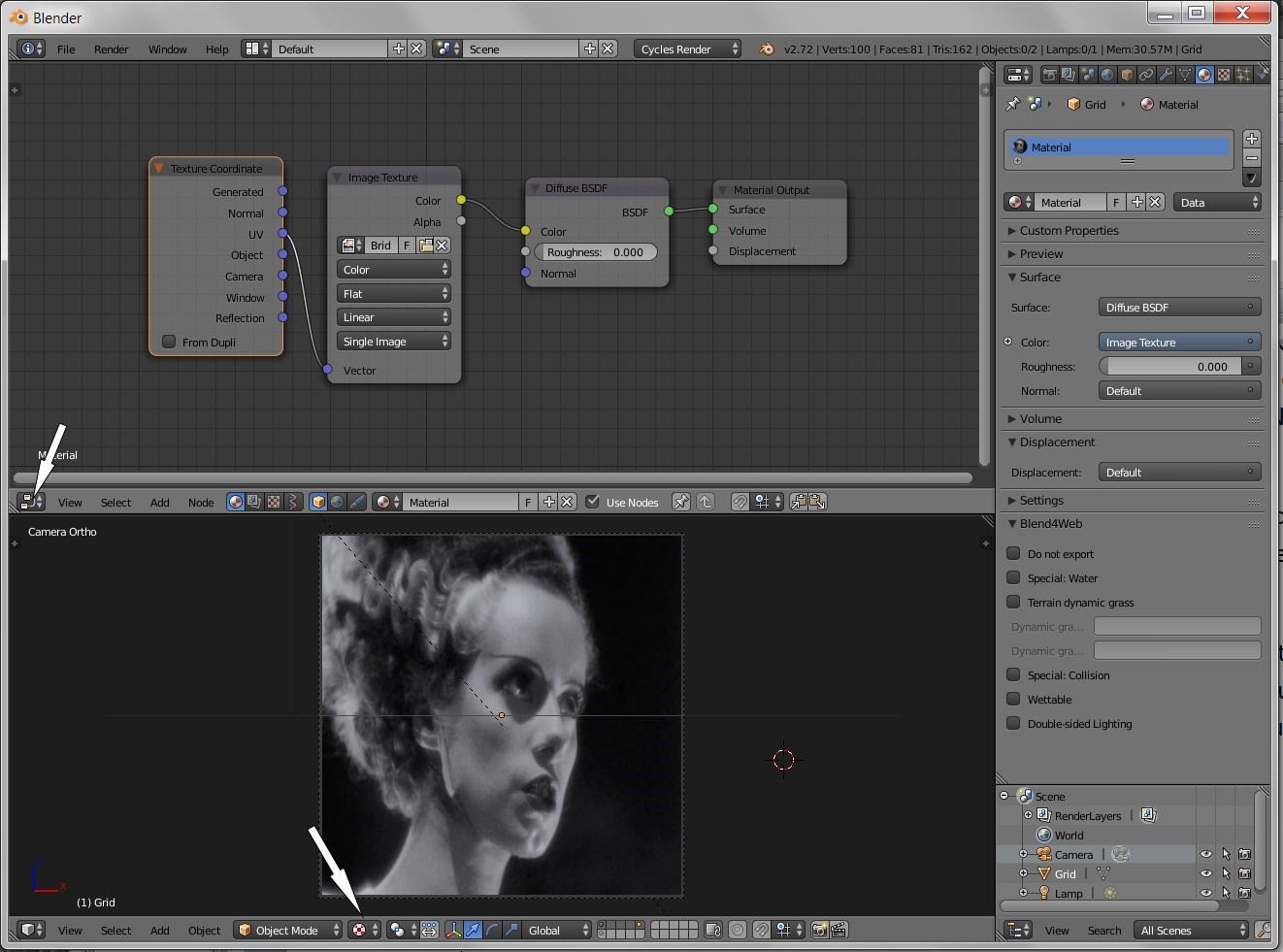
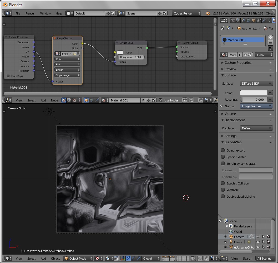
Let’s look at the image before it is glitched. Assign the image to the grid as a texture. I’ll go into a little more detail about the process later, but the following screenshot shows the node setup (please note.. we are using the Cycles renderer here, not Blender Internal!). Be sure to set the display view of the 3d pane to rendered or textured. Otherwise you’ll only see the plain, untextured grid. Mrs. Frankenstein is a little distorted here since she’s been mapped to a  perfect square.


02uvImageMapped

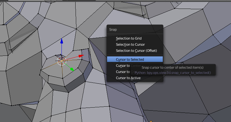
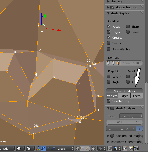
One more thing before we export our grid as an .obj file, let’s look at the UV vertices we just created. Go into “Edit” mode, select all the 3d vertices of the grid, then switch one of the panes to the “UV Image Editor”. You should see another grid that looks just like the 3d grid. To begin with, each of the UV vertices matches the position of it’s corresponding 3d vertex.


03.1uvNOTglitched

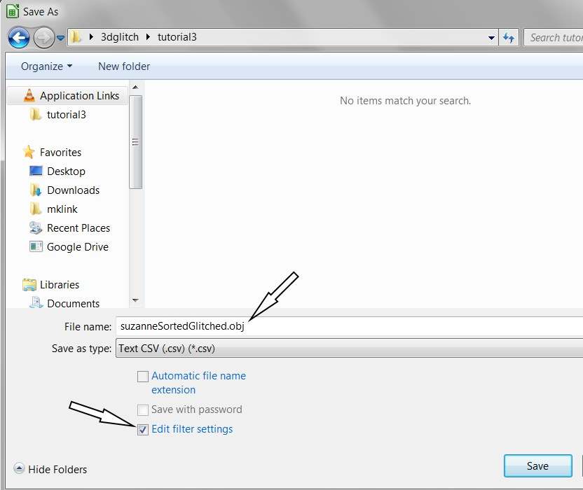
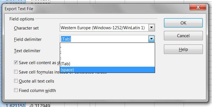
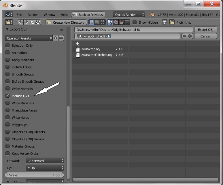
Next, export the grid as an .obj file as has been discussed in the earlier notes. Among the export options, be sure to check “Include UVs”.


03uvExportObj

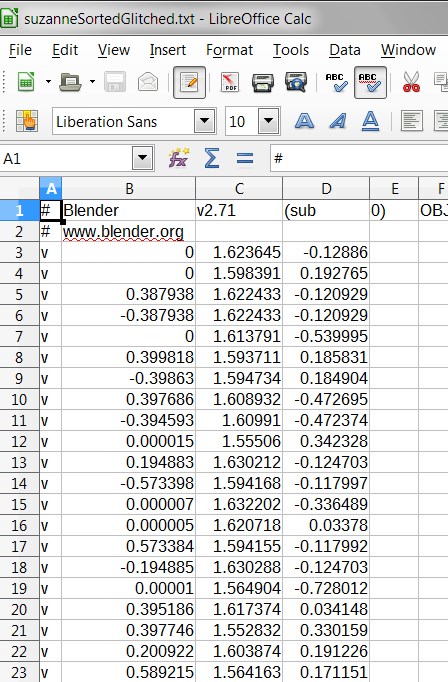
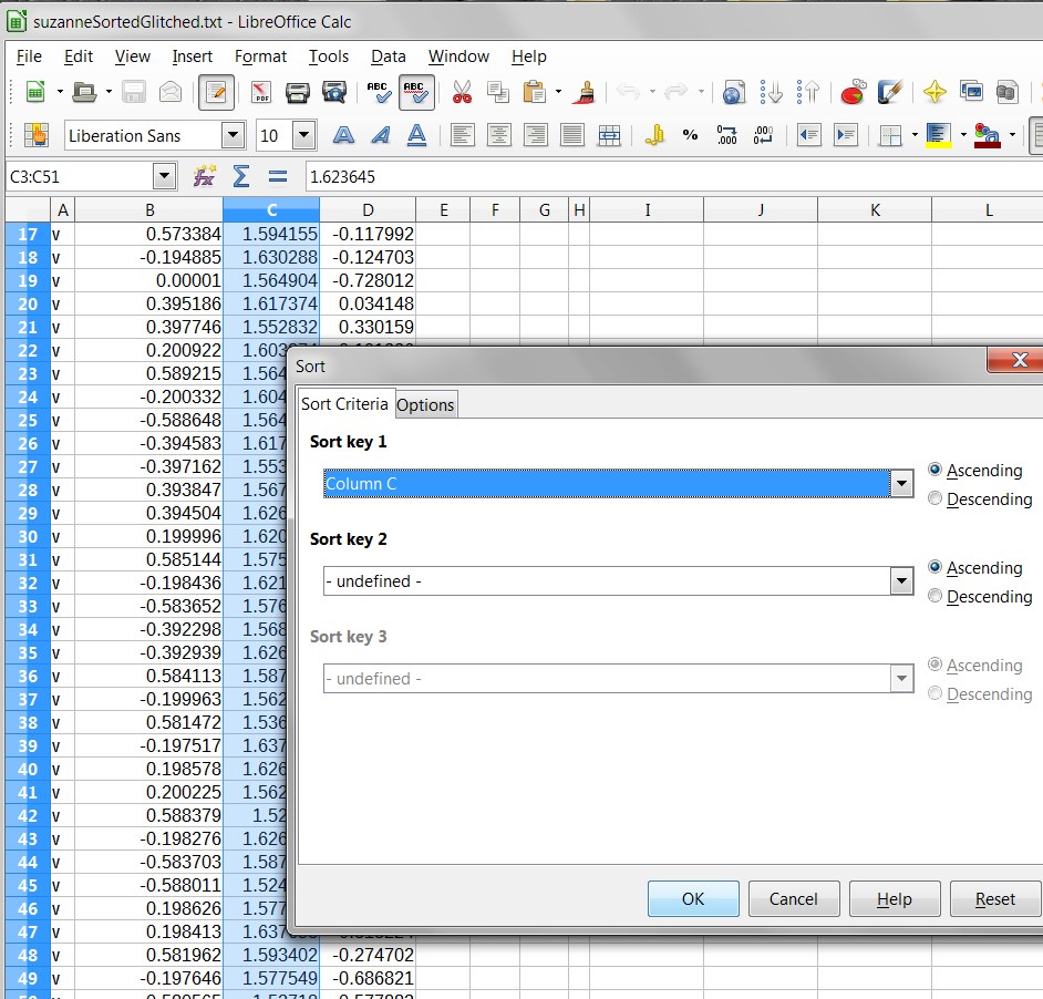
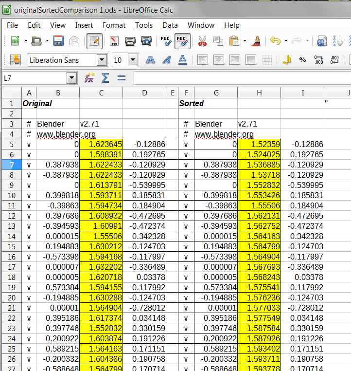
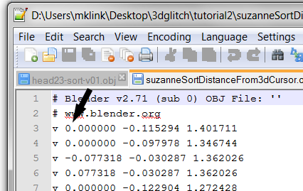
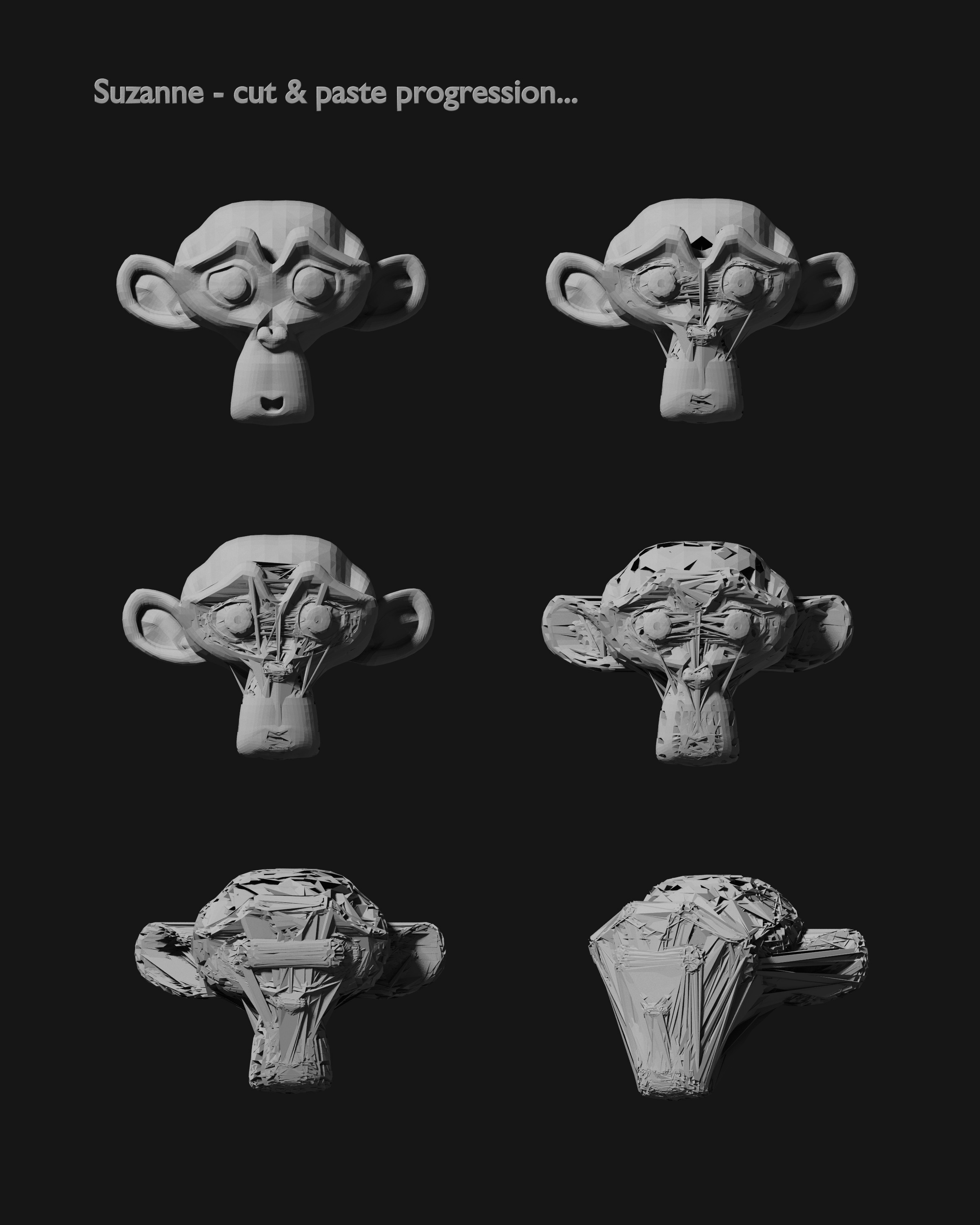
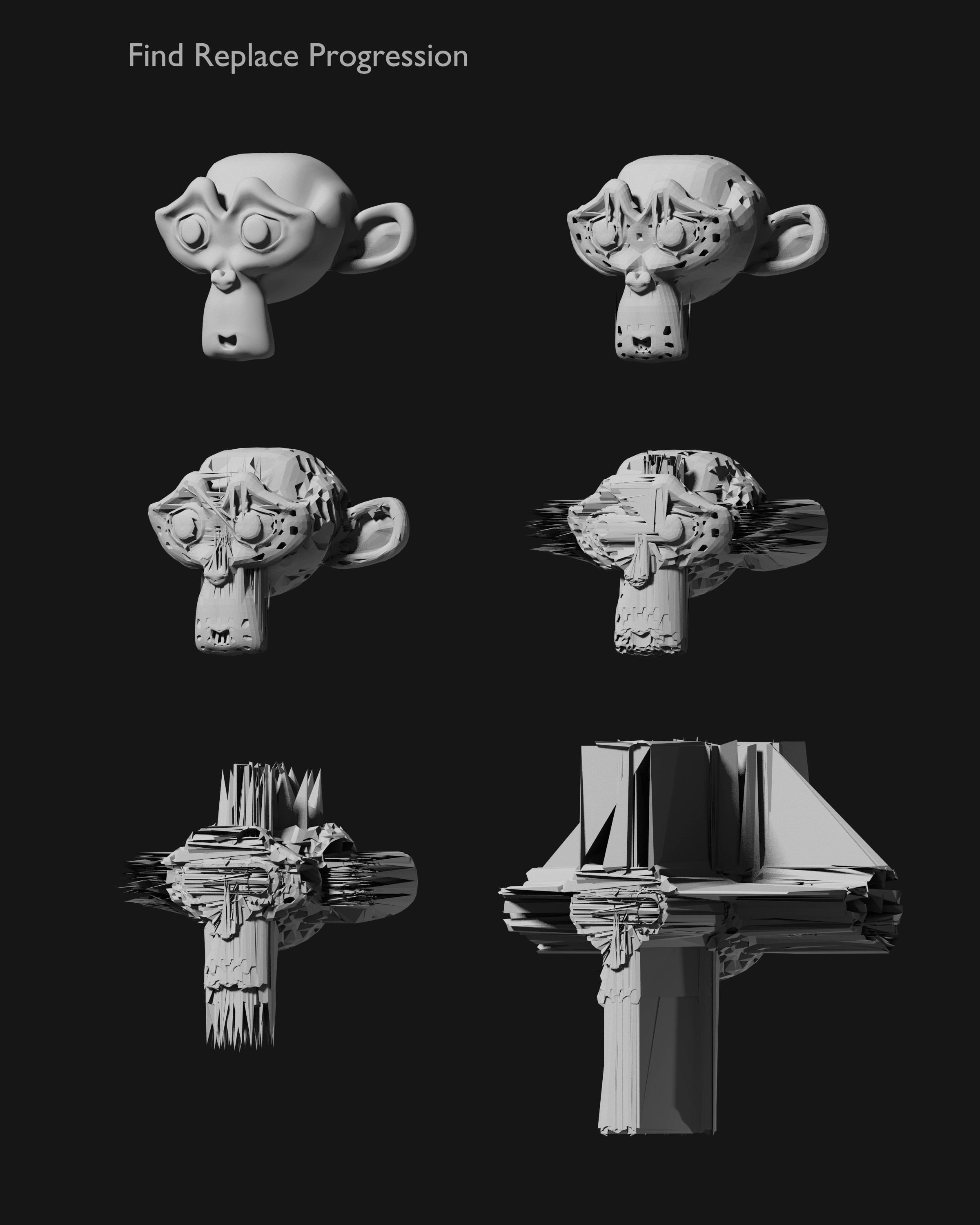
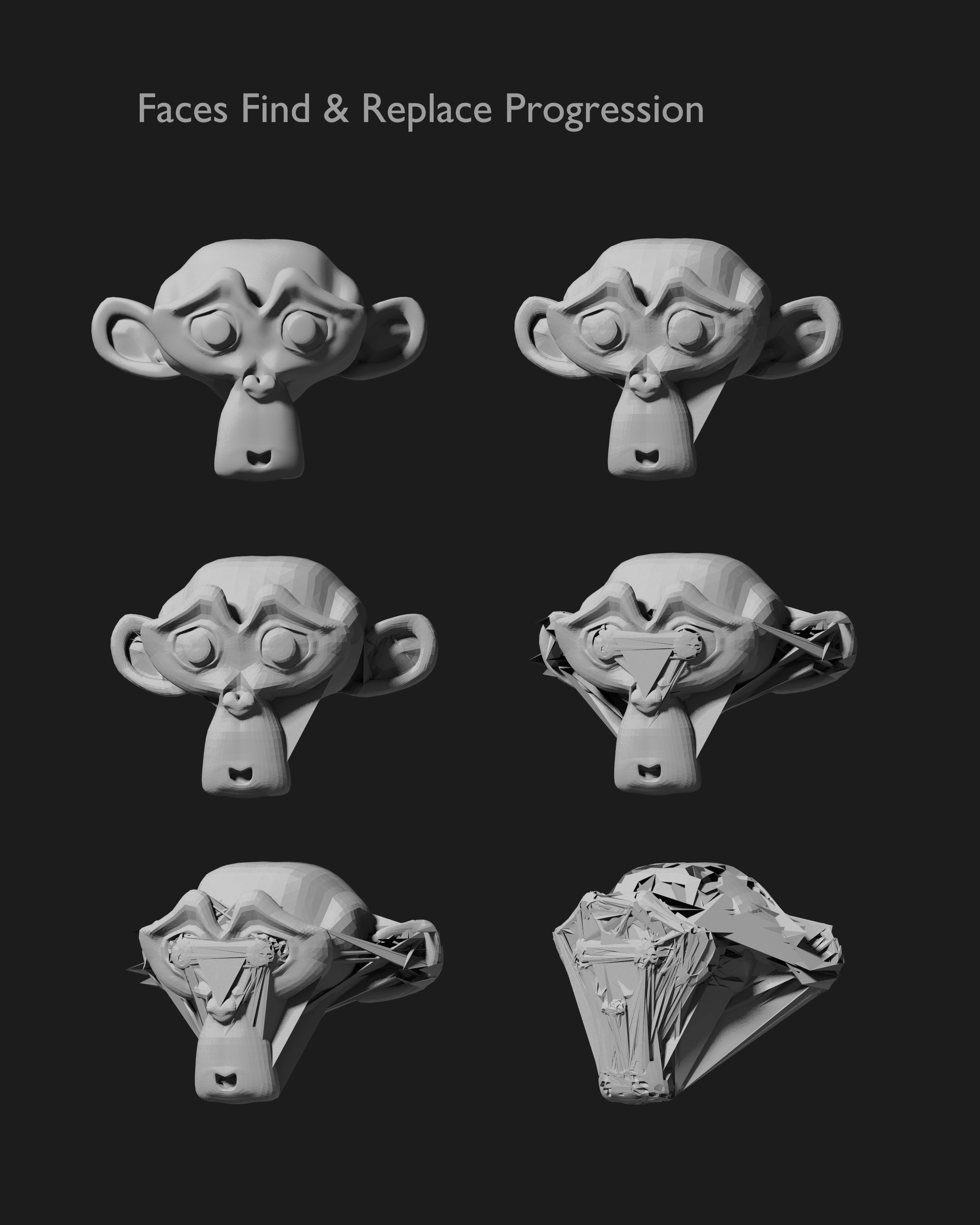
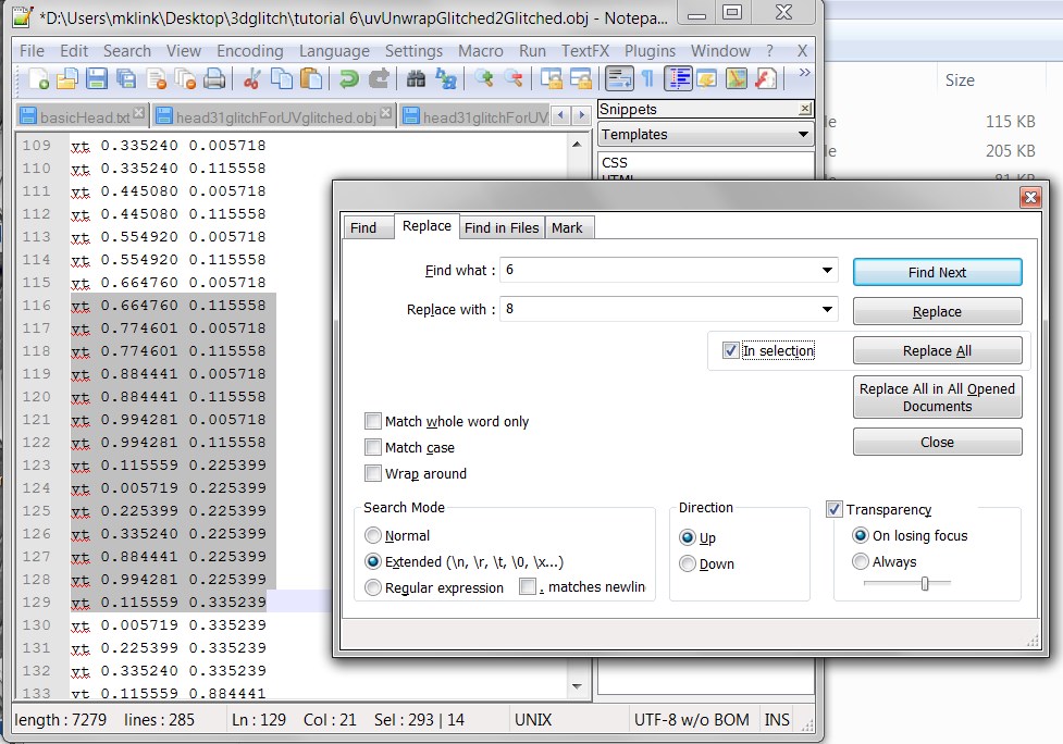
Next, open the resulting .obj file in a text editor or spreadsheet, again as described in the preceding notes. Go to the section with the lines beginning with “vt”, cut, paste, find and replace, while making sure that the total number of lines in the section remains the same.


04uvGlitch

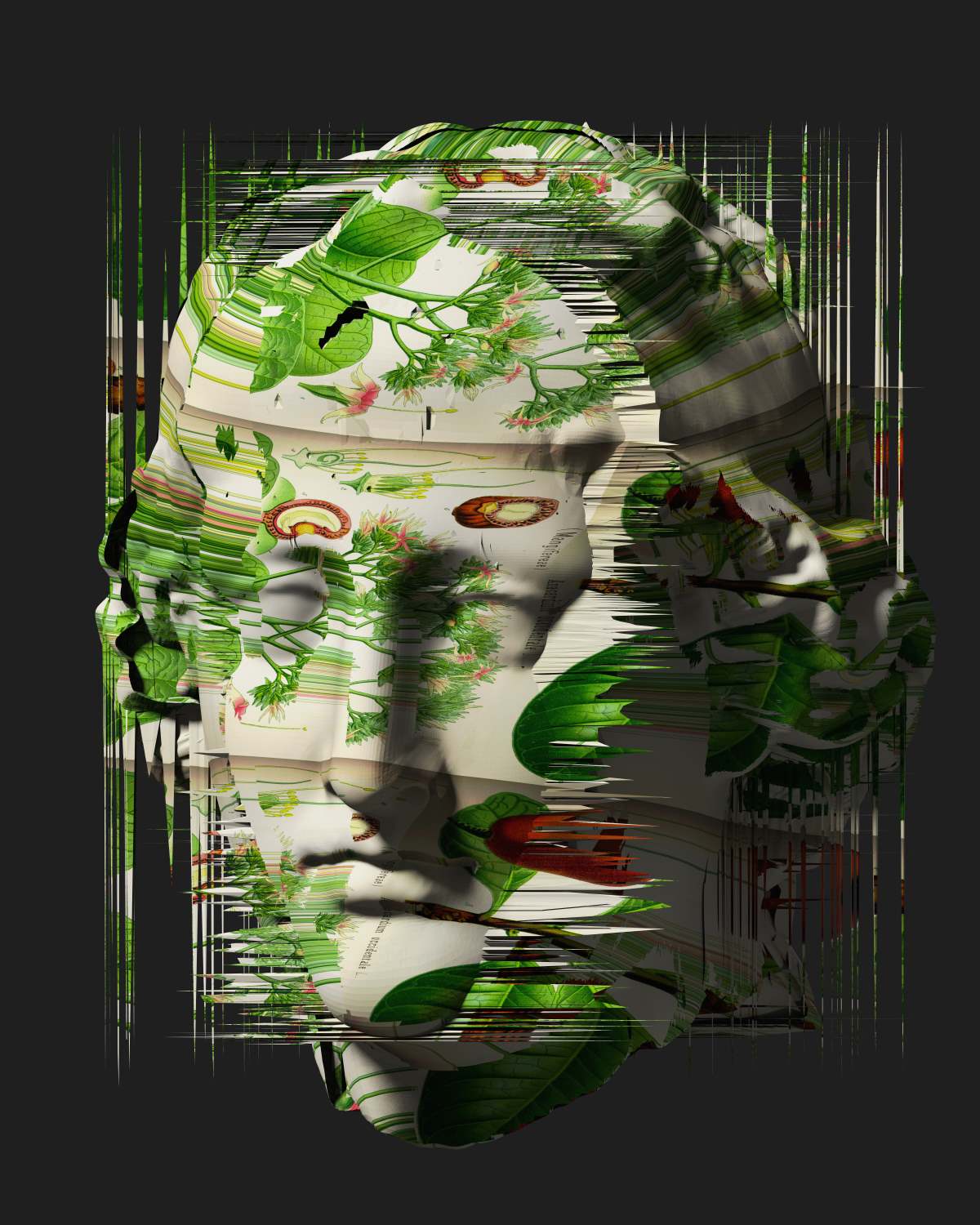
When you’re done and have saved your work, go back to Blender, import the glitched .obj file, and assign an image texture using the node system. The root node will be a Texture Coordinate node. Choose the “UV” feed. The next node will be a texture node. Choose “Image Texture” and load the image you want to map. The final node before the output will be a diffuse shader. Here, again, is a screenshot of the basic node setup.. Be sure to set the display mode of the 3d pane to textured or rendered: Notice how different Mrs. Frankenstein looks this time!


06uvsGlitchedReTextured

Let’s look at the UV vertices after the mangling they underwent while in the text editor. Go into Edit mode, select all the 3d vertices of the grid, and again switch one of the panes to the “UV Image Editor”


05uvsGlitchedReimport

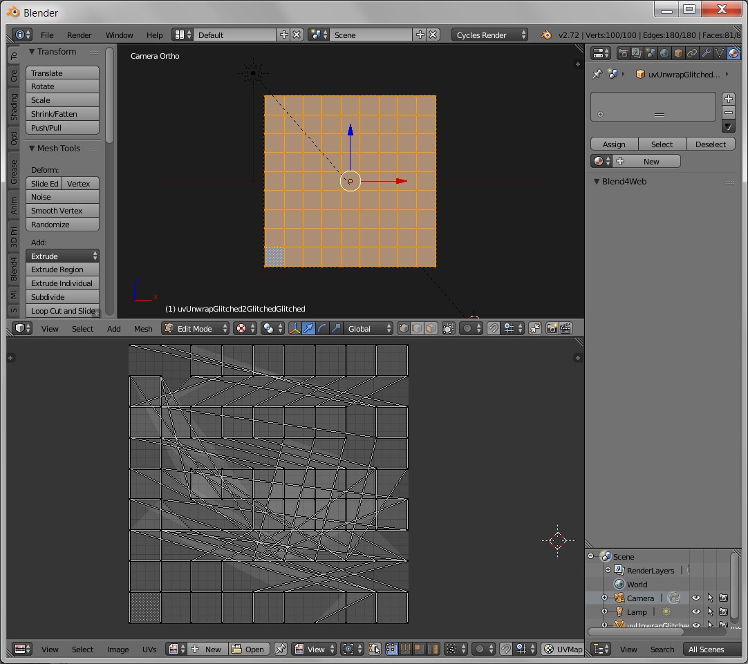
See how irregular the UV grid is now.. the mapping of the image has been thoroughly disrupted.

Note that the steps outlined above can be repeated until you are satisfied with the image. At that point you can do a final render as you would a normal 3d scene.


finalRender

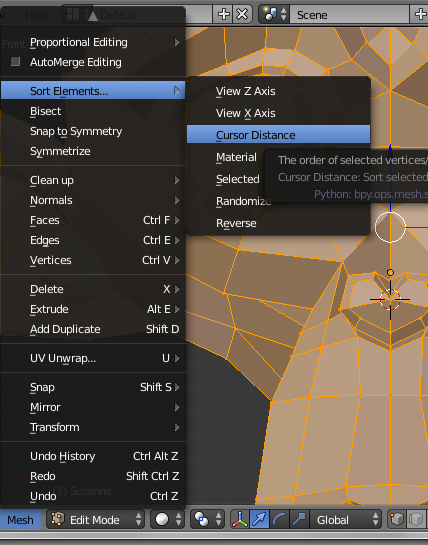
We’ve talked about how we can open the UV Image Editor and see the UVs.  What we haven’t mentioned is that  the UV coordinates can be directly manipulated in that editor, without going through the process of exporting to an .obj file for glitching.. that should give you a clue on how we can push this process further.

3d Glitching – Part 3

Again, this will go better if you’ve read part 1 and part 2 of this series!

We’re going to combine two techniques here. First, we’ll use the “Sort by Selection” method to order the vertices. Second, instead of using a text editor, we’ll use a spreadsheet to manipulate the data!!

We’ll use Suzanne, once again, as our model. We’ll go into “Edit” mode and  subdivide the mesh a couple times so we have more vertices to work with.

That accomplished, we’ll select a few of the vertices at the top of Suzanne’s head, and, after that, we’ll go to the “Mesh” menu, choose “Sort Elements”, and then sort by “Selection”.


Using the “visualize vertices” addon that we introduced in the last set of notes, we can now see that the vertices we selected are in indices 0 through 48 ( a total of 49).

4.1jpg

We then  export the mesh in our usual fashion as an .obj file, change the extension to .txt, and open it in a spreadsheet! I’m using LibreOffice Calc, so I’m given the option of using spaces to separate the fields, this results in the x,y, and z coordinates being placed correctly in their separate columns.


5

We’re now going to do something that would not have been possible using a text editor.  We’ll select the first 49 coordinates in the “C” column.. those represents the “y” values for the vertices, which is the “up” direction. ( A note here.. most 3d programs treat the “y” axis as up, but Blender  uses the “z” axis for up! When exporting as an .obj file from Blender, in the export options, choose “Y Up” and “Z Forward”.)


In this case, sort Column “C” by “Ascending”.


6

We’ve now “glitched” our file, but we have to take special care when saving it and changing it back into an .obj file. Choose to save as a text “.csv” file. In Calc, you’ll need to check the “Edit filter settings” option. You can also uncheck “Automatic file name extension” options, and then change the file extension from “.csv” to “.obj”.


7

Be sure to change the field delimiter to “space”:


8


We’ll now take a look at our glitched file in Meshlab:


9

Look at that strange regular pattern of  peaks and valleys on top of Suzanne’s head!  What is happening here?

Let’s look at a comparison of the column containing the values of the “y” coordinates before and after we sorted them:

6.1

Note that before we did our sort in the spreadsheet, the vertex at index 0  (on line 5 of the spreadsheet due to the header info above it) would be at the very top of Suzanne’s head.. at the highest “y” position. After we sorted the “y” axis in the spreadsheet in ascending order, that 0 index vertex was now at the lowest position on the “y” axis relative to the other vertices we selected.  Each of the subsequent vertices we selected would be at the next slightly higher position, and the last vertex at index 48 will now be at the highest relative position.

Let’s look again at the picture of the selected vertices with their index positions displayed.. this time with a visualization of the distribution of those indices:


4.1withArrows


Note how the pattern skips, hopscotch fashion, so the next indexed vertex is never immediately “spatially” adjacent in the mesh to the vertices that are just before and after it in the index order.

The “hopscotch” arrangement of the vertices results in the regular “high-low” alternation along the “y” axis that we see saw above. After the sort in the spreadsheet, the vertices reached during the first half of the traverse have all been assigned the lowest “y” values, and the vertices spatially in between them on the mesh, being visited last, have been assigned the highest “y” values. Of course, the order of the indices would have been different if we’d chosen a different method of sorting them back when we were in Blender.

This method of selecting chunks of the 3 columns representing the x, y, and z coordinates, and then sorting them various ways – sometimes ascending, sometimes descending, sometimes sorting one column separately, sometimes sorting more than one column using multiple keys – can produce some interesting results:

aphrodite003resized

There are many other curious things one can do with spreadsheets.. easily cutting and pasting between the columns, applying formulas.. however, sooner or later the limitations of spreadsheets will get in the way. At that point we’ll need to use a real scripting language to manipulate the date.. but that will come in a future post.

Before that, though, we’ll be looking at glitching the texture coordinates of the .obj file.. these control how a 2d image is mapped to the 3d surface of the mesh.. and now you’re ready to move on to the next section!

3d Glitch Notes.. Part 2

If you haven’t already.. be sure to read the first part of this series: 3d Glitching Part 1.   These notes assume that you already have an understanding of the material presented there, as well as an understanding of 3d modeling and the basic ideas behind “Glitch Art.”  In addition, some knowledge of the 3d modeling and rendering program “Blender” will be useful, since it will be the tool we’ll be using. We’ll be dealing with some of the more arcane features of Blender … I’ll sometimes provide a little extra explanation of Blender terminology in hopes that it will make it easier for users of other 3d modeling/rendering programs to follow and to make adjustments for their preferred environments.

This second set of notes provides a way to have some control over which areas of the model are “glitched.” As it is, the long list of vertices in an object file provides little information about what part of the model will be effected when we apply any of the techniques mentioned in part 1 – copy and paste or find and replace…  If the model was exported from Blender, the x, y, and z axis are likely all on a scale from 0.00000  to 1.00000 or -1.00000. If the information on a line for a particular vertex contains the coordinates -1.000000 -1.000000 1.000000, it might be at the extreme left, front, and top of the object (which coordinates are situated in the “minus” direction and which axes are”up” or “forward” depends on certain options chosen at the time of export.) However, the lines containing the positions of vertices and faces for an .obj file are often sorted in unpredictable or even completely random ways. Usually this is just fine.. it’s that unpredictability that makes glitch art so much fun!

However, there are times when you want more control.. you want to limit the “glitch” to a particular subsection of the model…

Blender provides a way to do just that. Within Blender we can choose to sort the vertices using several methods. Once you’ve sorted the vertices, when you export the model as an .obj file and open it in a text editor, you’ll find the vertex you’ve chosen as the starting point for your sort at the top of the list, with the remaining vertices more or less ordered according to their distance from that first vertex. If you want to “glitch” the area closest to that first vertex, then you copy/paste, etc. near the start of the list. If you want to avoid glitching that area, you perform your manipulations elsewhere in the list.

There are several sorting methods available, but  I’ve found two of them to be the most useful. The first is to sort the vertices according to their distance from the 3d cursor. The second is to sort by the selected vertices. We’ll start with the first of the two methods:

After having imported or created a model in Blender,  go into “Edit” mode. In Blender terminology that is when we can see and edit the individual vertices of the model. We’ll start by positioning the 3d cursor. You can simply place the cursor where you like by left-clicking with the mouse, but if you want it to align precisely with a particular vertex, select that vertex (using right-click) and then follow with the shift-s key combination to bring up the “Snap” menu, and choose “Cursor to Selected.”  Since we’re using Suzanne the Blender monkey for our model, let’s align the 3d cursor with the tip of her nose.


1-snap3dCursorToSelected

Once you’ve positioned the 3d cursor, select all the vertices, and then go to the “Mesh” menu, select “Sort Elements” and choose “Cursor Distance.”


2-sortDistanceTo3dCursor

However, it’s not clear at all from the normal Blender interface that anything has changed.. normally there is no indication of what the index of a given vertex is. In order to see the indices of vertices, you must  install the addon “3D View: Index Visualiser (BMesh)” which is available here: https://developer.blender.org/F11709 (There’s also a way to activate this feature by entering Blender into debug mode.. but the addon works better). (edit: there have been reports that this version of the addon no longer works.. if it doesn’t work for you, try this alternative:

 https://github.com/nutti/Index-Visualizer

You’ll have to look up the proper way to install third party addons into Blender .. however, I found that I had to extract the .py script. Simply installing from file and targeting the .zip did not seem to work.  Once the script is installed, you should find an “Index Visualizer” sub-panel in the “Properties” panel. Just click “Start” .. it automatically displays only the selected vertices…)

Once you’ve installed and activated the addon, you can go to the “Properties” panel, and then find and press the “Visualize Indices” button. You should then see the index of each vertex. I recommend that you choose the “Selected Only” and “Vertices” options so you can limit the information displayed. Otherwise the screen will be unreadable when dealing with a heavy mesh!


3-visualizeIndices

You’ll note that the vertex at the center of Suzanne’s nose has an index of 0 – That’s the vertex we used to position the 3d cursor. Don’t be confused by the appearance of index numbers that may seem to be in the “wrong” location, such as the “28” and “25” in the illustration above. the system displays the index numbers of vertices that are actually farther away, even when those vertices are hidden behind nearer polygons.

So we now have the vertices sorted according to their distance from the 3d cursor. At this point, we export the model as an .obj file, and then open the file in a text editor. Take a look at the following illustration:


4-TextEditorBefore

Note the x coordinate at 0.00000  – the nose was exactly in the center of Suzanne’s x axis! By sorting the vertices, the vertex at the tip of the nose, and the vertices closest to it have been brought to the top of the list. Now.. just to illustrate how it works, change that x coordinate to 2.00000, save the file, and then open in MeshLab. You should see the tip of the nose skewed far to the side:

5-MeshLabAfter

Of course it would be far simpler to just move that vertex manually within Blender. The point of all this is that knowing which vertices are at the top of the list, we can either target or avoid them when it comes to glitching. In the following illustration, the 3d cursor was placed at the tip of Suzanne’s right ear, and then the vertices were sorted according to their distance from the cursor. Then, when the exported .obj file was brought into the text editor, only vertices in the bottom half of the list were “glitched.” The result is that only the left half of Suzanne’s head is affected:


suzanneSorted-cropped

That’s it for today.. You are now ready to move on to part 3 of this series!

3d Glitching..

These notes presume that you have a basic understanding of glitching and of computer 3d modeling.

Instead of using standard 3d modeling tools to modify a shape, we’ll be directly manipulating the data in the file. Sometimes glitch artists employ a hex editor to accomplish this, but since the 3d file format we’re targeting is in ascii text, an ordinary text editor will do.

We’ll be using the Wavefront .obj file format. Models in this format are readily available on the web. However, I recommend that you use the open source modeling and rendering application Blender to either generate your own models or to simplify  third party models. Alternately, you can use Meshlab.

In Blender, export the model as an .obj file, but turn off all of the options – UVs, Materials, Normals, etc. etc. In Meshlab you will have similar options when exporting a mesh – we want only the most basic geometric information.

Once you have your file.. use your favorite text editor to open it. I’m currently using Windows, so the editor of choice for me is Notepad++.

In the editor, the file structure becomes easy to parse. The data for a simple cube, created in Blender and exported to .obj looks like this:

# Blender v2.71 (sub 0) OBJ File:
# www.blender.org

v -1.000000 -1.000000 1.000000
v -1.000000 -1.000000 -1.000000
v 1.000000 -1.000000 -1.000000
v 1.000000 -1.000000 1.000000
v -1.000000 1.000000 1.000000
v -1.000000 1.000000 -1.000000
v 1.000000 1.000000 -1.000000
v 1.000000 1.000000 1.000000

f 5 6 2 1
f 6 7 3 2
f 7 8 4 3
f 8 5 1 4
f 1 2 3 4
f 8 7 6 5


There’s no real header.. the part at the beginning is made up of notes, indicated by # signs.. the system disregards these. Next comes a list of vertices.. one for each line that begins with a “v”. Each of those lines contain three values for the x, y, z position of the vertex relative to the origin. The meaning of the scale may vary depending on the settings of the program you use. Blender typically operates in “Blender Units” . Our example is two Blender units along each edge (the distance from -1 to 0 and from 0 to 1), so a cube half the dimension of our example might have a vertex at position -0.5 -0.5 0.5

Next comes a list of polygons, referred to as “faces”, one on each line that begins with an “f”. In our example the faces are quads since they have four integer values, each integer indicating a vertex from the first part of the file. The integer corresponds to the index of the vertex. For example, the first quad of our cube is made up of the 5th, 6th, 2nd, and 1st vertices in the list. This structure will have important consequences when we begin to “glitch” the data.

We’ll first consider glitching the vertex data. One way to do this is to cut and paste. This changes the index of each vertex. The result is that some of the faces in the second part of the file no longer refer to the same vertices they did originally. Usually this means that the “glitched” form stays fairly close to the general outline of the original object.. we have all the same vertices – there are no vertices that have moved to new positions outside of the original object.. but the faces may be scrambled in curious ways. Note the following progression:


suzanneCutPasteProgressionProcessed

We’re using the famous Blender “Suzanne” monkey head as our model. Successive versions represents more drastic applications of cut and paste. At the beginning we use smaller snippets and paste them at positions that are closer to their original location. Later in the series we cut bigger chunks and paste them much farther away from their original location.

Another option is to use “Find and Replace” within the list of vertices. For example, one could search for all instances of “1” and replace it with “8”. This may result in more dramatic reshaping of the model. For example, a vertex that was originally at x axis -1.0000 would now be at x axis -8.0000 . That would mean that the vertex is now eight times further from the origin than its original position. Also, one might replace negatives with positives and vice versa. This would result in a displacement of the vertex in a direction opposite of its original position relative to the origin. See the following examples… again there is a progression from smaller changes to more dramatic ones.. starting out with find and replace over small subsets of the vertices and smaller differences between the number being replaced and the number replacing it. Toward the end, search and replace occurs over a wider span of the vertices and there are greater differences between the originals and the replacements:


findReplaceProgressionProcessed

Note that replacing a larger number with a smaller number generally results in a vertex that is inset.. that moves closer to the origin (assuming that the origin is at the center of the object.) For example, if we replace “8” with “2”, a vertex that was at Y axis -0.8 is now at -0.2, and a vertex that was at Y axis 0.8 will now be at 0.2 – in both the negative and the positive case the vertex ends up closer to the origin. Conversely, replacing a smaller number with a larger results in vertices that are farther away from the origin.

Another option is to change the part of the list that contains data for the faces. Cutting and pasting whole lines for each face will not have any effect.. it doesn’t matter what order the faces are in! If they refer to the same vertices they did before they will look exactly the same.

Finding and replacing integers within the lines will have an effect.. but you must be careful! This is where you are more likely to make the file unreadable… be sure that the result of your “find and replace” is not a reference to a vertex that does not exist. Recall that the vertices are indicated by their index number. If you have 1000 vertices and you replace “1” with “9”, you’ll end up with a reference to a non-existent vertex at position 9000. You should be safe if you always replace a larger number with a smaller number. (This is an area where a more intelligent script would be useful.. but that’s a topic for another day..) Here’s an example of finding and replacing the data in the “faces” section of the file.. as before, there’s a progression from fairly limited to more drastic replacements.


faceSearchReplaceProgressionProcessed

Obviously, one can combine all three of these techniques when “glitching” the file.

There are more advanced methods. In Blender one can specify a vertex that will be the starting point for sorting the vertices. Thus one could force the vertices at the tip of Suzanne’s nose to come at the start of the list. This allows some control of where the glitching will take place. If one knows that the nose of the figure is at the beginning of the list, one could avoid changing data in that area if the object was to preserve the original form of the nose.

Now that you’ve finished this first section, move on the the second set of notes, here.

Hello World

After years of neglect, I’ve revived my ancient website. I’ve given in to convenience.. no more hand coding.. just standard blog software.. so, hopefully, the ease of it all will result in more frequent updating..

For now, all I have to point out are the galleries that are either on the right or below… my various 3d art works…


head007-small
One of my heads…